Dyd's Blog

He who has a strong enough why can bear almost any how.

扫描线

不只是线段树的那个……

扫描线

普通

虽然线段树那里已经学过一点扫描线了,但还是问一问:

给定一些矩形,求其面积并

这个太简单了,直接跳过了

进阶

看这个:

给定一些三角形,求其面积并

分析

三角形比矩形讨厌的地方在于,矩形平行于坐标轴,只用考虑四个顶点,但三角形可以斜着

考虑把三角形用顶点和交点划分,如图:

三角

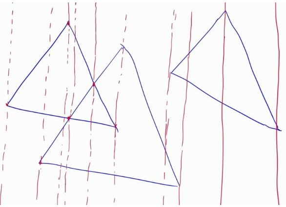
每两个红色的线之间不存在边的交点,换句话说,都是梯形(广义上的),直接两边线段长度求并,乘高除以二即可

由于三角形有 $n$ 个,两两间都可能有交点,故时间复杂度为 $O(N^3)$

注意三角形有边和扫描线重合的特判,排序即可

代码

三角形面积并

大量使用 STL 的后果是,不开 O2 TLE 一个点,开了直接飞过去

1
2
3
4
5
6
7
8
9
10
11
12
13
14
15
16
17
18
19
20
21
22
23
24
25
26
27
28
29
30
31
32
33
34
35
36
37
38
39
40
41
42
43
44
45
46
47
48
49
50
51
52
53
54
55
56
57
58
59
60
61
62
63
64
65
66
67
68
69
70
71
72
73
74
75
76
77
78
79
80
81
82
83
84
85
86
87
88
89
90
91
92
93
94
95
96
97
98
99
100
101
#include <bits/stdc++.h>
#define fi first
#define se second
#define pb emplace_back
using DB = double;
using PDD = std::pair<double, double>;
const int N = 100 + 10;
const DB eps = 1e-8, INF = 0x3f3f3f3f;
std::array<PDD, 3> tr[N];
PDD q[N];
int n, top;
int cmp(DB x, DB y)
{
if (std::fabs(x - y) < eps) return 0;
return x > y ? 1 : -1;
}
PDD operator + (PDD x, PDD y){ return {x.fi + y.fi, x.se + y.se}; }
PDD operator - (PDD x, PDD y){ return {x.fi - y.fi, x.se - y.se}; }
PDD operator * (PDD x, DB y){ return {x.fi * y, x.se * y}; }
PDD operator / (PDD x, DB y){ return {x.fi / y, x.se / y}; }
DB operator & (PDD x, PDD y){ return x.fi * y.fi + x.se * y.se; }
DB operator * (PDD x, PDD y){ return x.fi * y.se - x.se * y.fi; }
bool on(PDD p, PDD x, PDD y){ return cmp((p - x) & (p - y), 0) <= 0; }
PDD jiao(PDD x, PDD u, PDD y, PDD v)
{
if (!cmp(u * v, 0)) return {INF, INF};
DB t = v * (x - y) / (u * v);
PDD o = x + u * t;
if (!on(o, x, x + u) || !on(o, y, y + v)) o = {INF, INF};
return o;
}
DB bot(DB x, bool side)
{
top = 0;
for (int i = 0; i < n; ++i)
{
auto t = tr[i];
if (cmp(t[0].fi, x) > 0 || cmp(t[2].fi, x) < 0) continue;
if (!cmp(t[0].fi, x) && !cmp(t[1].fi, x))
{
if (side) q[top++] = {t[0].se, t[1].se};
continue;
}
if (!cmp(t[1].fi, x) && !cmp(t[2].fi, x))
{
if (!side) q[top++] = {t[1].se, t[2].se};
continue;
}
DB d[3];
int u = 0;
for (int j = 0; j < 3; ++j)
{
PDD o = jiao(t[j], t[(j + 1) % 3] - t[j], {x, -INF}, {0, INF * 2});
if (cmp(o.fi, INF)) d[u++] = o.se;
}
if (!u) continue;
std::sort(d, d + u);
q[top++] = {d[0], d[u - 1]};
}
if (!top) return 0;
for (int i = 0; i < top; ++i) if (q[i].fi > q[i].se) std::swap(q[i].fi, q[i].se);
std::sort(q, q + top);
DB res = 0, st = q[0].fi, ed = q[0].se;
for (int i = 1; i < top; ++i)
if (q[i].fi <= ed) ed = std::max(ed, q[i].se);
else
{
res += ed - st;
st = q[i].fi, ed = q[i].se;
}
res += ed - st;
return res;
}
DB calc(DB x, DB y){ return (bot(x, true) + bot(y, false)) * (y - x) / 2; }
int main()
{
scanf("%d", &n);
std::vector<DB> xs;
for (int i = 0; i < n; ++i)
{
for (int j = 0; j < 3; ++j)
{
scanf("%lf %lf", &tr[i][j].fi, &tr[i][j].se);
xs.pb(tr[i][j].fi);
}
std::sort(tr[i].begin(), tr[i].end());
}
for (int i = 0; i < n; ++i)
for (int j = 0; j < i; ++j)
for (int p = 0; p < 3; ++p)
for (int q = 0; q < 3; ++q)
{
PDD o = jiao(tr[i][p], tr[i][(p + 1) % 3] - tr[i][p], tr[j][q], tr[j][(q + 1) % 3] - tr[j][q]);
if (cmp(o.fi, INF)) xs.pb(o.fi);
}
std::sort(xs.begin(), xs.end());
DB ans = 0;
for (int i = 0; i + 1 < xs.size(); ++i) if (cmp(xs[i], xs[i + 1])) ans += calc(xs[i], xs[i + 1]);
printf("%.2lf\n", ans);
return 0;
}

炼狱

解决了三角形,就相当于解决了所有多边形(剖分成三角性即可),可正当你得意都时候,圆来了

圆咋办?如果扫描线的话那个弧形可不好求,没有办法,为了对付大boss,只好祭出大杀器——自适应辛普森积分

辛普森积分

先看看辛普森积分是神马

顾名思义,这是一种积分方法,来看下面这个函数:

函数

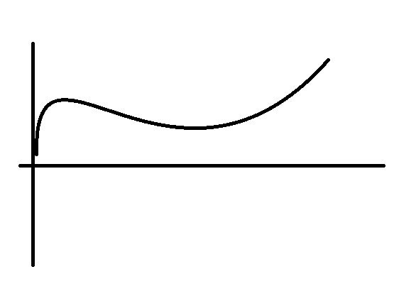
求面积当然是用积分了,但它的解析式又很麻烦,咋办?

辛普森提出一个玄妙的方法:把他近似成一个二次函数

js

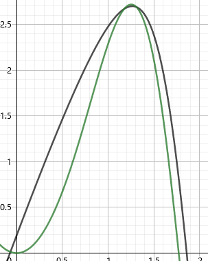
如图,直接把绿色曲线当成黑色的二次函数积分,设绿色曲线为 $y = f(x)$ ,取 $(l, f(l)), (r, f(r)), (mid, f(mid))$ 三个点确定这个黑色的二次函数

二次函数的积分就很好求了,就是:
$$
\frac{f(l) + f(mid) * 4 + f(r)}{6} * (r - l)
$$

自适应

解决了辛普森,来看看自适应

显然直接辛普森积分是无法满足精度要求的,我们要让他“适应”我们设定的精度,具体地,对于区间 $[l, r]$ ,设其辛普森积分后面积为 $S$ ,而区间 $[l, mid], [mid, r]$ 辛普森积分的面积为 $L, R$ ,若 $|L + R - S| < eps$ ,我们就认为这个积分到达了要求的精度;否则,递归积分左右两边,加起来即可

代码

自适应辛普森积分

1
2
3
4
5
6
7
8
9
10
11
12
13
14
15
16
17
18
19
20
21
22
23
24
25
26
27
#include <bits/stdc++.h>
#define DB double
using namespace std;
const DB eps = 1e-12;
DB f(DB x)
{
return sin(x) / x;
}
DB simpson(DB l, DB r)
{
return (r - l) * (f(l) + f((l + r) / 2) * 4 + f(r)) / 6;
}
DB asr(DB l, DB r, DB s)
{
DB mid = (l + r) / 2;
DB L = simpson(l, mid), R = simpson(mid, r);
if (fabs(L + R - s) < eps)
return L + R;
return asr(l, mid, L) + asr(mid, r, R);
}
int main()
{
DB l, r;
scanf("%lf %lf", &l, &r);
printf("%lf\n", asr(l, r, simpson(l, r)));
return 0;
}

圆的面积并

辛普森积分的应用一般是更改 f 函数:

圆的面积并

1
2
3
4
5
6
7
8
9
10
11
12
13
14
15
16
17
18
19
20
21
22
23
24
25
26
27
28
29
30
31
32
33
34
35
36
37
38
39
40
41
42
43
44
45
46
47
48
49
50
51
52
53
54
55
56
57
58
59
60
61
62
63
64
65
66
67
68
69
70
71
72
#include <bits/stdc++.h>
#define DB double
using namespace std;
const int N = 1000 + 5;
const DB eps = 1e-8;
int n;
struct Point
{
DB x, y;
bool operator < (const Point &t) const
{
return x == t.x ? y < t.y : x < t.x;
}
} q[N];
struct Circle
{
Point p;
DB r;
} c[N];
int cmp(DB x, DB y)
{
if (fabs(x - y) < eps)
return 0;
return x > y ? 1 : -1;
}
DB f(DB x)
{
int cnt = 0;
for (int i = 0; i < n; ++i)
{
DB X = fabs(x - c[i].p.x), R = c[i].r;
if (cmp(X, R) < 0)
{
DB Y = sqrt(R * R - X * X);
q[cnt++] = {c[i].p.y - Y, c[i].p.y + Y};
}
}
if (!cnt)
return 0;
sort(q, q + cnt);
DB res = 0, st = q[0].x, ed = q[0].y;
for (int i = 1; i < cnt; i++)
if (q[i].x <= ed)
ed = max(ed, q[i].y);
else
{
res += ed - st;
st = q[i].x, ed = q[i].y;
}
return res + ed - st;
}
DB simpson(DB l, DB r)
{
return (r - l) * (f(l) + f((l + r) / 2) * 4 + f(r)) / 6;
}
DB asr(DB l, DB r, DB s)
{
DB mid = (l + r) / 2;
DB L = simpson(l, mid), R = simpson(mid, r);
if (fabs(L + R - s) < eps)
return L + R;
return asr(l, mid, L) + asr(mid, r, R);
}
int main()
{
scanf("%d", &n);
for (int i = 0; i < n; ++i)
scanf("%lf %lf %lf", &c[i].p.x, &c[i].p.y, &c[i].r);
DB l = -2000, r = 2000;
printf("%.3lf\n", asr(l, r, simpson(l, r)));
return 0;
}

再看一道题

上面两道是以前做的,码风略差,来看这个:

【模板】自适应辛普森法 2

一看,这个函数没法直接积分(不像模板1可以硬艹),就只有自适应辛普森,好消息是显然 $x \to \infty$ 时函数值趋近于 $0$ ,但一个问题是,何时此函数发散?

结论是: $a < 0$ 时,原函数发散

什么,推倒?小小年纪不学好天天就想着推倒别人!啥,还要看推倒过程!你你你,这在我国是违法的啊!

呃呃,还是给大家 推倒 推导一下

首首先,随便去网上找一个收敛准则:

极限比较判别法

对于正项级数 $\{a_n\}, \{b_n\}$ ,有 $\lim_{n \to \infty} \frac{a_n}{b_n} = c$ :

  1. 若 $c = \infty$ 且 $\sum b_n$ 发散,则 $\sum a_n$ 发散
  2. 若 $c = 0$ 且 $\sum b_n$ 收敛,则 $\sum a_n$ 收敛
  3. 若 $c$ 为常数,则 $\sum a_n$ , $\sum b_n$ 同时收敛或发散

然后我们来看这个东西,假设原积分在 $x_0$ 处发散(以下 $\int$ 都不写范围)
$$
\begin{aligned}
& \lim_{x \to x_0} \frac{x^{\frac{a}{x} - x}}{x} \\
= & \lim_{x \to x_0} x^{\frac{a}{x} - x - 1} \\
= & \lim_{x \to x_0} e^{\frac{a}{x} - x - 1 \ln x} \\
= & e^{\lim_{x \to x_0} \frac{a}{x} - x - 1 \ln x} \\
\end{aligned}
$$
显然 $\int x$ 是发散的,我们想让 $\int x^{\frac{a}{x} - x}$ 发散,那么就要上式 $= \infty$ ,而如果 $x \to \infty$ (显然 $x \ge 0$ ),那么无论 $a$ 如何取上式都为 $0$ ;所以为了让上式 $= \infty$ , $x \to 0$ ,此时如果 $a < 0$ 则上式 $= \infty$ ,由极限比较判别法可知, $\int x^{\frac{a}{x} - x}$ 发散

什么?你还想推倒收敛?色胆包天,我我我,我要报警了

开玩笑,下面 推倒 推导 $a \ge 0$ 时必收敛,其实差不多

还是上面的法则:
$$
\begin{aligned}
& \lim_{x \to x_0} \frac{x^{\frac{a}{x} - x}}{\frac{1}{x}} \\
= & e^{\lim_{x \to x_0} \frac{a}{x} - x + 1 \ln x} \\
\end{aligned}
$$
然后就不用我多说了吧?

1
2
3
4
5
6
7
8
9
10
11
12
13
14
15
16
17
18
19
20
#include <bits/stdc++.h>
using DB = double;
const DB eps = 1e-8;
DB a;
DB f(DB x){ return std::pow(x, a / x - x); }
DB sim(DB l, DB r){ return (r - l) * (f(l) + f((l + r) / 2) * 4 + f(r)) / 6; }
DB asr(DB l, DB r, DB s)
{
DB mid = (l + r) / 2, t;
DB ls = sim(l, mid), rs = sim(mid, r);
if (std::fabs(t = (ls + rs - s)) <= eps * 15) return ls + rs + t / 15;
return asr(l, mid, ls) + asr(mid, r, rs);
}
int main()
{
scanf("%lf", &a);
if (a < 0) puts("orz");
else printf("%.5lf\n", asr(eps, 20, sim(eps, 20)));
return 0;
}

然后你会想问 $11$ 行是个啥玩意?其实这是一个公式:
$$
\mid \int_a^b f(x)dx - S(a_1, b_1) - S(a_2, b_2) \mid \approx \frac{1}{15} \mid S(a_1, b_1) + S(a_2, b_2) - S(a, b) \mid
$$